July 2021 – Statpacking

Does Bayesian statistical analysis involve stronger assumptions compared to frequentist statistical analysis? It is commonly believed that the answer is yes because frequentist analysis makes assumptions about the likelihood while Bayesian analysis requires assumptions on both the likelihood and the prior. Since priors are absent from frequentist analysis, it seems reasonable to say that Bayesian analysis needs more assumptions compared to frequentist analysis. Quite a few statisticians distrust modeling assumptions on the grounds that they are fundamentally unverifiable and these statisticians are much more sceptical about Bayesian methods compared to frequentist ones.

I held similar views until not too long ago but have realized recently that the nature of assumptions underlying frequentist and Bayesian analyses is quite different and it is not at all clear to me anymore that frequentist analysis indeed makes fewer assumptions. In fact, from the likelihood standpoint, Bayesian analysis makes much fewer assumptions compared to frequentist analysis. Specifically, in Bayesian analysis, one needs to model only the probability of observing the given dataset at hand conditional on the unknown parameter while in frequentist analysis, one typically needs to model, for every possible imaginary dataset, the probability of observing that dataset. I will try to illustrate this here using the following elementary problem in statistical inference that is surely familiar to every statistics student.

Problem: Suppose a scientist makes ${6}$ numerical measurements 26.6, 38.5, 34.4, 34, 31, 23.6 of an unknown physical quantity ${\theta}$ . On the basis of these measurements, what can be inferred about ${\theta}$ ?

Standard frequentist and Bayesian approaches to this problem are described below and they lead to identical solutions which allows for a transparent comparison of the assumptions underlying the two approaches. I will assume below that all involved random variables have densities.

Let me start with a detailed description of the standard frequentist approach. The observed dataset here consists of the ${n = 6}$ points ${x_1^{\text{obs}} = 26.6}$ , ${x_2^{\text{obs}} = 38.5}$ , ${x_3^{\text{obs}} = 34.4}$ , ${x_4^{\text{obs}} = 34}$ , ${x_5^{\text{obs}} = 31}$ , ${x_6^{\text{obs}} = 23.6}$ . One can consider any other set of ${6}$ real numbers ${x_1, \dots, x_6}$ as an imaginary alternative dataset. One can presumably also allow alternative datasets to have different numbers of points. The collection of all such imaginary alternative datasets is known as the sample space whose specification is essential to frequentist inference. We shall take the sample space to be the set of all ${6}$ real numbers ${x_1, \dots, x_6}$ . If the scientist used a stopping criterion to obtain their data (such as, for example, the criterion of stopping as soon as a measurement less than 25 is observed), then this simple sample space will not work (we would need to allow datasets with varying lengths in that case).

Freq-Step 1: The observed values ${x_1^{\text{obs}}, \dots, x_n^{\text{obs}}}$ are assumed to be realizations of random variables ${X_1, \dots, X_n}$ .

Freq-Step 2: ${X_1,\dots, X_n}$ are assumed to be independently distributed according to the normal distribution with mean ${\theta}$ (which is the unknown quantity of interest) and an unknown variance ${\sigma^2}$ . Mathematically, this means that ${X_1,\dots, X_n}$ have the joint probability density function:

$\displaystyle f_{X_1, \dots, X_n}(x_1, \dots, x_n) = \left(\frac{1}{\sqrt{2 \pi} \sigma} \right)^n \exp \left(-\frac{1}{2 \sigma^2} \sum_{i=1}^n \left(x_i - \theta \right)^2 \right) ~~ \text{for all real numbers} ~x_1, \dots, x_n. \ \ \ \ \ (1)$

The above assumption describes the probability of obtaining every possible imaginary dataset in the sample space.

Freq-Step 3: Under assumption (1), it is a well-known mathematical fact that ${\sqrt{n} \left(\bar{X} - \theta \right)/S}$ has the Student ${t}$ -distribution with ${n-1}$ degrees of freedom where $\displaystyle \bar{X} := \frac{X_1 + \dots + X_n}{n} ~~ \text{ and } ~~ S := \sqrt{\frac{1}{n-1} \sum_{i=1}^n \left(X_i - \bar{X} \right)^2}.$

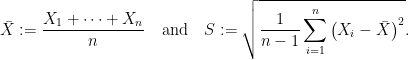
Freq-Step 4: Because of the distributional result of Freq-Step 3,

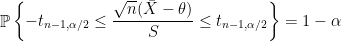
$\displaystyle \mathop{\mathbb P} \left\{-t_{n-1, \alpha/2} \leq \frac{\sqrt{n} (\bar{X} - \theta)}{S} \leq t_{n-1, \alpha/2} \right\} = 1 - \alpha$ for every ${\alpha \in (0, 1)}$

where ${t_{n-1, \alpha/2}}$ is the ${(1 - \alpha/2)}$ -quantile of the Student ${t}$ -distribution with ${n-1}$ degrees of freedom. This is equivalent to saying that ${\theta}$ is contained in the random interval

$\displaystyle \left[\bar{X}-t_{n-1, \alpha/2} \frac{S}{\sqrt{n}}, \bar{X} + t_{n-1, \alpha/2} \frac{S}{\sqrt{n}} \right] ~~ \text{with probability}~ 1-\alpha. \ \ \ \ \ (2)$

Freq-Step 5: The observed values corresponding to ${x_1^{\text{obs}}, \dots, x_n^{\text{obs}}}$ and ${n = 6}$ are plugged in (2) and the interval is calculated explicitly. With the values listed in the problem, we get $\displaystyle [31.35 - t_{5, \alpha/2} (2.238), 31.35 + t_{5, \alpha/2} (2.238)]$ as the ${100(1-\alpha) \%}$ confidence interval for ${\theta}$ . The common choice ${\alpha = 0.05}$ leads to the ${95\%}$ confidence interval ${[25.598, 37.102]}$ .

So the frequentist approach required a specification of the sample space and the precise assumption (1) of the probability of observing every possible imaginary dataset in the sample space. If we only make the assumption (1) for a subset of datasets in the sample space, the distributional fact in Freq-Step 3 will no longer hold. An alternative frequentist approach based on asymptotics to this problem would make, instead of (1), the assumption that ${X_1, \dots, X_n}$ are independent and identically distributed according to a distribution with mean ${\theta}$ and a finite variance ${\sigma^2}$ :

$\displaystyle f_{X_1, \dots, X_n}(x_1, \dots, x_n) = \sigma^{-n} g \left(\frac{x_1 - \theta}{\sigma} \right) \dots g \left(\frac{x_n - \theta}{\sigma} \right) ~~\text{for all real numbers}~ x_1, \dots, x_n \ \ \ \ \ (3)$

for some density function ${g}$ satisfying ${\int x g(x) dx = 0}$ and ${\int x^2 g(x) dx = 1}$ . This is a more general assumption compared to (1) but it still needs to hold for all ${x_1, \dots, x_n}$ i.e., for all possible imaginary elements of the sample space.

Let us now look at the standard Bayesian approach before comparing the two approaches.

Bayes-Step 1: The observed values ${x_{1}^{\text{obs}}, \dots x_n^{\text{obs}}}$ are assumed to be realizations of random variables ${X_1, \dots, X_6}$ . The unknown physical quantity ${\theta}$ is also considered to be random from the point of view of the scientist/data analyst who is uncertain about its actual value. The goal is to calculate the conditional density of ${\theta}$ given ${X_1 = x_1^{\text{obs}}, \dots, X_n = x_n^{\text{obs}}}$ :

$\displaystyle f_{\theta | X_1 = x_1^{\text{obs}}, \dots, X_n = x_n^{\text{obs}}}(z) ~~\text{for all values of}~ z.$ .

Bayes rule is applied to give

$\displaystyle f_{\theta | X_1 = x_1^{\text{obs}}, \dots, X_n = x_n^{\text{obs}}}(z) \propto f_{X_1, \dots, X_n \mid \theta = z}(x_1^{\text{obs}}, \dots, x_n^{\text{obs}}) f_{\theta}(z) \ \ \ \ \ (4)$

where the ${\propto}$ sign means that the left hand side is equal to the right hand side multiplied by a factor that does not depend on ${z}$ (the factor does depend on ${x_1^{\text{obs}}, \dots, x_n^{\text{obs}}}$ ). Modeling assumptions are needed for ${f_{X_1, \dots, X_n|\theta}(x_1^{\text{obs}}, \dots, x_n^{\text{obs}})}$ (likelihood) and ${f_{\theta}(\cdot)}$ (prior).

Bayes-Step 2: For the likelihood model, a parameter ${\sigma}$ is introduced for the scale of the noise in the measurements so one can write

$\displaystyle f_{X_1, \dots, X_n|\theta}(x_1^{\text{obs}}, \dots, x_n^{\text{obs}}) = \int_0^{\infty} f_{X_1, \dots, X_n|\theta, \sigma = s}(x_1^{\text{obs}}, \dots, x_n^{\text{obs}}) f_{\sigma|\theta}(s) ds.$

It is assumed that

$\displaystyle f_{X_1, \dots, X_n|\theta, \sigma}(x_1^{\text{obs}}, \dots, x_n^{\text{obs}}) = \left(\frac{1}{\sqrt{2 \pi} \sigma} \right)^n \exp \left(-\frac{1}{2 \sigma^2} \sum_{i=1}^n \left(x^{\text{obs}}_i - \theta \right)^2 \right). \ \ \ \ \ (5)$

${f_{\sigma|\theta}(\cdot)}$ and ${f_{\theta}(\cdot)}$ can together be considered as prior specification and, for these, it is assumed that

$\displaystyle f_{\sigma|\theta}(s) = \frac{1}{s}I\{s > 0\} ~ \text{ for all } s ~~ \text{ and } ~~ f_{\theta}(z) = 1 ~\text{ for all } z \ \ \ \ \ (6)$

for all ${s}$ and ${z}$ respectively. These are improper priors.

Bayes-Step 3: Plugging in (6) and (5) in (4), we get

$\displaystyle f_{\theta | X_1 = x_1^{\text{obs}}, \dots, X_n = x_n^{\text{obs}}}(z) \propto \int_0^{\infty} \frac{1}{s^{n+1}} \exp \left(-\frac{1}{2s^2} \sum_{i=1}^n \left(x_i^{\text{obs}} - \theta\right)^2 \right) ds.$

One can pull out the term involving ${\theta}$ by a simple change of variable resulting in

$\displaystyle f_{\theta | X_1 = x_1^{\text{obs}}, \dots, X_n = x_n^{\text{obs}}}(z) \propto \left(\sum_{i=1}^n \left(x_i^{\text{obs}} - \theta\right)^2 \right)^{-n/2} \propto \left(1 + \frac{1}{n-1} \frac{(\bar{x}^{\text{obs}} - \theta)^2}{\left(s^{\text{obs}}/\sqrt{n} \right)^2} \right)^{-n/2}$

where

$\displaystyle \bar{x}^{\text{obs}} := \frac{x^{\text{obs}}_1 + \dots + x^{\text{obs}}_n}{n} ~~ \text{ and } ~~ s^{\text{obs}} := \sqrt{\frac{1}{n-1} \sum_{i=1}^n \left(x^{\text{obs}}_i - \bar{x}^{\text{obs}} \right)^2}.$

One can check with the formula for the density of the ${t}$ -distribution that the above is equivalent to

$\displaystyle \frac{\sqrt{n} \left(\bar{x}^{\text{obs}} - \theta \right)}{S^{\text{obs}}} \biggr\rvert X_1 = x_1^{\text{obs}}, \dots, X_n = x_n^{\text{obs}}$

having the student ${t}$ -distribution with ${n-1}$ degrees of freedom.

Bayes-Step 4: Because of the distributional result in Bayes-Step 3,

$\displaystyle \mathop{\mathbb P} \left\{-t_{n-1, \alpha/2} \leq \frac{\sqrt{n} \left(\bar{x}^{\text{obs}} - \theta \right)}{S^{\text{obs}}} \leq t_{n-1, \alpha/2} \biggr\rvert X_1 = x_1^{\text{obs}}, \dots, X_n = x_n^{\text{obs}} \right\} = 1-\alpha$

which is equivalent to saying that, conditional on ${X_1 = x_1^{\text{obs}}, \dots, X_n = x_n^{\text{obs}}}$ , the random variable ${\theta}$ is contained in the fixed interval

$\displaystyle \left[\bar{x}^{\text{obs}}-t_{n-1, \alpha/2} \frac{s^{\text{obs}}}{\sqrt{n}}, \bar{x}^{\text{obs}} + t_{n-1, \alpha/2} \frac{s^{\text{obs}}}{\sqrt{n}} \right] ~~ \text{ with probability} ~ 1 - \alpha. \ \ \ \ \ (7)$

Bayes-Step 5: The observed values corresponding to ${x_1^{\text{obs}}, \dots, x_n^{\text{obs}}}$ and ${n = 6}$ are plugged in (7) and the interval is calculated explicitly. With the values listed in the problem, we get

$\displaystyle [31.35 - t_{5, \alpha/2} (2.238), 31.35 + t_{5, \alpha/2} (2.238)]$

as the ${100(1-\alpha) \%}$ credible interval for ${\theta}$ . The common choice ${\alpha = 0.05}$ leads to the ${95\%}$ credible interval ${[25.598, 37.102]}$ .

The Bayes analysis which leads to identical answers as the frequentist analysis relies on the assumption (6) for the prior and the assumption (5) for the likelihood. Let us now compare these with the assumptions (1) (and (3)) underlying frequentist analysis:

Priors: Bayesian analysis uses the assumption (6) on the prior densities and, of course, there are no such assumptions in frequentist analysis. In this particular case, the prior assumptions are reasonable and principled arguments (based on invariant transformations) exist to justify them as a valid mathematical representation of the state of complete ignorance on part of the scientist/data analyst about ${\theta}$ and ${\sigma}$ outside of the observed data (see Chapter 12 of the book Probability theory: the logic of science by E. T. Jaynes).

Likelihood: The frequentist likelihood assumption is (1) while the Bayesian likelihood assumption is (5). Clearly (1) is much stronger than (5) as the former requires equality at all ${x_1, \dots, x_n}$ while the latter requires equality only at ${x_1^{\text{obs}}, \dots, x_n^{\text{obs}}}$ . From the Bayesian viewpoint, imaginary unobserved datasets ${x_1, \dots, x_n}$ are irrelevant to the problem at hand as one conditions on ${X_1 = x_1^{\text{obs}}, \dots, X_n = x_n^{\text{obs}}}$ throughout the analysis. From the frequentist viewpoint however, alternative datasets become relevant and one needs explicit assumptions on probabilities of observing them. Many textbooks write the Bayesian likelihood assumption as $\displaystyle X_1, \dots, X_n \mid \theta, \sigma \overset{\text{i.i.d}}{\sim} N(\theta, \sigma^2).$ This should be avoided as it refers to (1) while the actual Bayesian assumption is the much weaker (5). As I already mentioned, the ${t}$ -distribution result in Freq-Step 3 cannot be obtained using the much weaker assumption (5).

More on likelihood: Let us now compare the alternative frequentist likelihood assumption (3) with (5). These cannot be directly compared but one can still note that (3) is assumed for all ${x_1, \dots, x_n}$ while (5) is only for the observed dataset. Besides, frequentist analysis under the assuption (3) relies on asymptotics by sending the sample size ${n}$ to ${\infty}$ and (3) is a very strong assumption (although it is weaker than (1)) when ${n}$ is large; indeed, how does one know that a high-dimensional density can be written in that product form for all ${x_1, \dots, x_n}$ ? One cannot use any asymptotic results such as the central limit theorem under the Bayesian likelihood assumption (5).

As functions of ${\theta}$ and ${\sigma}$ : One may argue that as a function of the parameters, (1) is weaker compared to (5) because (1) only needs to hold for the true values of ${\theta}$ and ${\sigma}$ while (5) needs to hold for all ${\theta}$ and ${\sigma}$ . This is true in the example provided here but frequentist analysis also usually considers likelihoods as functions of the parameters (for example, while calculating maximum likelihood estimators).

Strong assumptions are usually easy to invalidate and (1) can be invalidated easily when ${n}$ is large (the histogram of the observed data ${X_1, \dots, X_n}$ can be plotted and checked for closeness to a normal distribution). The assumption (3) is more complicated and people just assume that it must be true (but it is still a strong assumption because it needs to hold for all points in the sample space). On the other hand, how does one invalidate the very weak Bayesian likelihood assumption (5)?

An interesting aspect of the specific problem considered here is that both the frequentist and Bayesian approaches lead to the same answer. Specifically, both approaches assert that ${\theta \in [25.598, 37.102]}$ . Now ${\theta}$ is a fixed physical constant that either lies in the interval ${[25.598, 37.102]}$ or does not. In spite of this, one would like to associate a probability of 0.95 to the proposition ${\theta \in [25.598, 37.102]}$ . From a Bayesian perspective, this is not a problem because the scientist/data analyst solving this problem is uncertain about the proposition ${\theta \in [25.598, 37.102]}$ and any uncertainty can be quantified by a conditional probability (here the conditioning event is ${X_1 = x_1^{\text{obs}}, \dots, X_n = x_n^{\text{obs}}}$ ). From a frequentist point of view however, there is no meaning to the statement: “ ${\theta \in [25.598, 37.102]}$ holds with probability 0.95″ because this proposition is either always true or always false and it cannot be given any meaning in terms of repeated trials. To salvage this problem, the frequentist goes to the statement which produced this interval:

$\displaystyle \theta \in \left[\bar{X}-t_{n-1, \alpha/2} \frac{S}{\sqrt{n}}, \bar{X} + t_{n-1, \alpha/2} \frac{S}{\sqrt{n}} \right]. \ \ \ \ \$

This statement (written in terms of the random variables ${X_1, \dots, X_n}$ themselves instead of their observed values) can indeed be assigned a probability by the frequentist. This probability assignment is with respect to the random variables ${X_1, \dots, X_n}$ so the frequentist is thus forced to consider other values that ${X_1, \dots, X_n}$ could have taken but have not taken in this specific observed dataset. Such a need for considering imaginary alternative datasets does not arise in Bayesian analyses.

To summarize this post, frequentist methods make much more stringent assumptions on the probability of observing data compared to Bayesian methods. On the other hand, Bayesian methods involve prior assumptions which frequentist methods have no need for. Which analysis are you more comfortable with?

Monthly Archives: July 2021

Who makes stronger assumptions: Bayesians or Frequentists?