Le Cam’s Hypothesis Testing Inequality

My first post is about a beautiful hypothesis testing inequality due to Le Cam [1, Chapter 16, Section 4]. Here is the setting. There is an unknown distribution ${P}$ on which we have two hypotheses. The first hypothesis is ${H_0 : P \in \mathcal{P}_0}$ and the second is ${H_1: P \in \mathcal{P}_1}$ where ${\mathcal{P}_0}$ and ${\mathcal{P}_1}$ denote classes of probability measures. Given i.i.d data ${X_1, \dots, X_n}$ from ${P}$ , the goal is to figure out which of the two hypothesis is the right one.

As one gets more and more data points i.e., as ${n}$ increases, this problem intuitively should get easier. Le Cam’s inequality quantifies this by asserting that the error in this hypothesis testing problem decreases exponentially in ${n}$ . The precise statement and a proof sketch of this inequality is given below. This inequality has many applications; a particularly interesting one is its role in establishing frequentist convergence rates of posterior distributions; this will be outlined in a future post.

We first need to specify the notion of error in hypothesis testing. Given a test ${\phi}$ (which is simply a ${[0, 1]}$ -valued function of the data), its type I error is ${\sup_{P \in \mathcal{P}_0} \mathop{\mathbb E}_P \phi(X_1, \dots, X_n)}$ while its type II error is ${\sup_{P \in \mathcal{P}_1} \mathop{\mathbb E}_P \left( 1 - \phi(X_1, \dots, X_n)\right) }$ . For ease of notation, let me write ${P^n \phi}$ for ${\mathop{\mathbb E}_P\phi(X_1, \dots, X_n)}$ where ${P^n}$ is the ${n}$ -fold product of ${P}$ with itself. We define the error of a test ${\phi}$ to be the sum of its type I and type II errors. 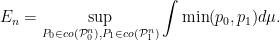The smallest error in testing ${H_0}$ against ${H_1}$ is therefore

$\displaystyle E_n := \inf_{\phi} \sup_{P_0 \in \mathcal{P}_0, P_1 \in \mathcal{P}_1} P_0^n \phi + P_1^n (1 - \phi).$

Le Cam’s inequality states that ${E_n}$ decreases exponentially in ${n}$ . The rate of this decrease depends on how close the classes ${\mathcal{P}_0}$ and ${\mathcal{P}_1}$ are. This closeness is measured by the so-called Hellinger affinity between ${\mathcal{P}_0}$ and ${\mathcal{P}_1}$ defined as

$\displaystyle \rho(\mathcal{P}_0, \mathcal{P}_1) := \sup_{P_0 \in \mathcal{P}_0, P_1 \in \mathcal{P}_1} \int \sqrt{p_0 p_1} d\mu$

where ${p_0}$ and ${p_1}$ denote the densities of ${P_0}$ and ${P_1}$ with respect to a common dominating measure ${\mu}$ . ${\int \sqrt{p_0 p_1} = 1 - \int (\sqrt{p_0} - \sqrt{p_1})^2/2}$ measures closeness between ${P_0}$ and ${P_1}$ with large values indicating closeness. Hence the name affinity.

The precise statement of Le Cam’s inequality is

$\displaystyle E^{1/n}_n \leq \rho \left(co(\mathcal{P}_0), co(\mathcal{P}_1) \right) \ \ \ \ \ (1)$

where ${co(\mathcal{P}_0)}$ denotes the convex hull of ${\mathcal{P}_0}$ i.e., the class of all finite linear combinations of probability measures in ${\mathcal{P}_0}$ . As a consequence, we have that ${E_n}$ decreases exponentially in ${n}$ as long as ${\rho(co(\mathcal{P}_0), co(\mathcal{P}_1))}$ is bounded from above by a constant strictly smaller than one. It must be noted that (1) is a finite sample result i.e., it is allowed that ${\mathcal{P}_0}$ and ${\mathcal{P}_1}$ depend on ${n}$ . It might seem strange that (1) involves the convex hulls of ${\mathcal{P}_0}$ and ${\mathcal{P}_1}$ instead of ${\mathcal{P}_0}$ and ${\mathcal{P}_1}$ themselves. This can be explained perhaps by the simple observation: ${\sup_{P \in \mathcal{P}} P \phi = \sup_{P \in co(\mathcal{P})} P \phi}$ .

Let me now provide a sketch of the proof of (1). Let ${\mathcal{P}_0^n := \{P^n : P \in \mathcal{P}_0\}}$ and similarly define ${\mathcal{P}_1^n}$ . Rewrite ${E_n}$ as

$\displaystyle E_n = \inf_{\phi} \sup_{P_0 \in \mathcal{P}^n_0, P_1 \in \mathcal{P}_1^n} \left(P_0 \phi + P_1 (1 - \phi)\right).$

The first idea is to interchange the inf and sup above. This is formally done via a minimax theorem. See this note by David Pollard for a clear exposition of a minimax theorem and its application to this particular example. This gives

$\displaystyle E_n = \sup_{P_0 \in co(\mathcal{P}^n_0), P_1 \in co(\mathcal{P}^n_1)} \inf_{\phi}\left(P_0 \phi + P_1 (1 - \phi)\right).$

Minimax theorems require the domains (on which the inf and sup are taken) to be convex which is why one gets convex hulls above. The advantage of using the minimax theorem is that the infimum above can be easily evaluated explicitly. This is because

$\displaystyle P_0 \phi + P_1 (1 - \phi) = \int \left(p_0 \phi + p_1 (1 - \phi) \right) d\mu \geq \int \min(p_0, p_1) d\mu.$

We thus get

$\displaystyle E_n = \sup_{P_0 \in co(\mathcal{P}_0^n), P_1 \in co(\mathcal{P}_1^n)} \int \min(p_0, p_1) d\mu.$

The quantity ${\int \min(p_0, p_1) d\mu}$ also measures closeness between ${P_0}$ and ${P_1}$ . It is actually called the total variation affinity between ${P_0}$ and ${P_1}$ . The trouble with it is that it is difficult to see how the right hand side above changes with ${n}$ . This is the reason why one switches to Hellinger affinity. The elementary inequality ${\min(a, b) \leq \sqrt{ab}}$ gives

$\displaystyle E_n \leq \sup_{P_0 \in co(\mathcal{P}_0^n), P_1 \in co(\mathcal{P}_1^n)} \int \sqrt{p_0 p_1} d\mu = \rho \left( co(\mathcal{P}_0^n), co(\mathcal{P}_1^n) \right).$

The proof is now completed by showing that

$\displaystyle \rho \left( co(\mathcal{P}_0^n), co(\mathcal{P}_1^n) \right) \leq \rho \left(co(\mathcal{P}_0), co(\mathcal{P}_1) \right)^n. \ \ \ \ \ (2)$

This inequality is a crucial part of the proof. This is the reason why one works with Hellinger affinity as opposed to the total variation affinity although the latter is more directly related to ${E_n}$ . Let us see why (2) holds when ${n = 2}$ . The general case can be tackled similarly.

Any probability measure in ${co(\mathcal{P}_0^2)}$ is of the form ${A = \sum_i \alpha_i P^2_{i0}}$ for some ${P_{i0} \in \mathcal{P}_0}$ . Similarly, any probability measure in ${co(\mathcal{P}_1^2)}$ is of the form ${B = \sum_j \alpha_j P^2_{j1}}$ for some ${P_{j1} \in \mathcal{P}_1}$ . The Hellinger affinity between ${A}$ and ${B}$ is therefore

$\displaystyle \int \int \sqrt{\sum_{i} \alpha_i p_{i0}(x) p_{i0}(y)} \sqrt{\sum_j \beta_j p_{j1}(x) p_{j2}(y)} d\mu(x) d\mu(y).$

Now if ${m_0(x) := \sum_{i} \alpha_i p_{i0}(x)}$ and ${m_1(x) := \sum_j \beta_j p_{j1}(x)}$ , we can rewrite the above as

$\displaystyle \int \sqrt{m_0(x)} \sqrt{m_1(x)} \left[ \int \sqrt{\frac{\sum_{i} \alpha_i p_{i0}(x) p_{i0}(y)}{\sum_i \alpha_i p_{i0}(x)}} \sqrt{\frac{\sum_{j} \beta_j p_{j1}(x) p_{j1}(y)}{\sum_j \beta_j p_{j1}(x)}} d\mu(y)\right] d\mu(x).$

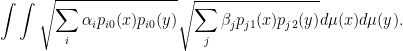
Fixing ${x}$ and looking at the inner integral above, the densities (as functions of ${y}$ ) involved are all convex combinations of densities in ${\mathcal{P}_0}$ and ${\mathcal{P}_1}$ respectively. Therefore the inner integral above is at most ${\rho(co(\mathcal{P}_0), co(\mathcal{P}_1))}$ which means that the above quantity is atmost

$\displaystyle \rho(co(\mathcal{P}_0), co(\mathcal{P}_1)) \int \sqrt{m_0(x) m_1(x)} d\mu(x).$

By the same logic, ${\int \sqrt{m_0 m_1} \leq \rho(co(\mathcal{P}_0), co(\mathcal{P}_1))}$ . This proves (2) for ${n = 2}$ . The general case is not much more difficult. This completes the sketch of the proof of (1).

References

[1] L. Le Cam. Asymptotic Methods in Statistical Decision Theory. Springer-Verlag, New York, 1986.

Le Cam’s Hypothesis Testing Inequality

Published by Aditya

Leave a Comment Cancel reply

Share this:

Related

Published by Aditya

Leave a Comment Cancel reply